Control Bootstrap Simulation Error
Source:R/bootstrap_helpers.R
estimate_boot_reps_for_target_cv.RdThis function estimates the number of bootstrap replicates needed to reduce the simulation error of a bootstrap variance estimator to a target level, where "simulation error" is defined as error caused by using only a finite number of bootstrap replicates and this simulation error is measured as a simulation coefficient of variation ("simulation CV").
Arguments
- svrepstat
An estimate obtained from a bootstrap replicate survey design object, with a function such as
svymean(..., return.replicates = TRUE)orwithReplicates(..., return.replicates = TRUE).- target_cv
A numeric value (or vector of numeric values) between 0 and 1. This is the target simulation CV for the bootstrap variance estimator.
Value
An object of class sim_cv_curve.
The functions summary(), plot(), and print() can be used on this object.
Call summary() to obtain a summary data frame.
The summary data frame has one row for each value of target_cv.
The column TARGET_CV gives the target coefficient of variation.
The column MAX_REPS gives the maximum number of replicates needed
for all of the statistics included in svrepstat. The remaining columns
give the number of replicates needed for each statistic.
Calling plot() produces a plot with 'ggplot2'.
Suggested Usage
- Step 1: Determine the largest acceptable level of simulation error for key survey estimates, where the level of simulation error is measured in terms of the simulation CV. We refer to this as the "target CV." A conventional value for the target CV is 5%.
- Step 2: Estimate key statistics of interest using a large number of bootstrap replicates (such as 5,000)
and save the estimates from each bootstrap replicate. This can be conveniently done using a function
from the survey package such as svymean(..., return.replicates = TRUE) or withReplicates(..., return.replicates = TRUE).
- Step 3: Use the function estimate_boot_reps_for_target_cv() to estimate the minimum number of bootstrap
replicates needed to attain the target CV.
Statistical Details
Unlike other replication methods such as the jackknife or balanced repeated replication, the bootstrap variance estimator's precision can always be improved by using a larger number of replicates, as the use of only a finite number of bootstrap replicates introduces simulation error to the variance estimation process. Simulation error can be measured as a "simulation coefficient of variation" (CV), which is the ratio of the standard error of a bootstrap estimator to the expectation of that bootstrap estimator, where the expectation and standard error are evaluated with respect to the bootstrapping process given the selected sample.
For a statistic \(\hat{\theta}\), the simulation CV of the bootstrap variance estimator
\(v_{B}(\hat{\theta})\) based on \(B\) replicate estimates \(\hat{\theta}^{\star}_1,\dots,\hat{\theta}^{\star}_B\) is defined as follows:
$$
CV_{\star}(v_{B}(\hat{\theta})) = \frac{\sqrt{var_{\star}(v_B(\hat{\theta}))}}{E_{\star}(v_B(\hat{\theta}))} = \frac{CV_{\star}(E_2)}{\sqrt{B}}
$$
where
$$
E_2 = (\hat{\theta}^{\star} - \hat{\theta})^2
$$
$$
CV_{\star}(E_2) = \frac{\sqrt{var_{\star}(E_2)}}{E_{\star}(E_2)}
$$
and \(var_{\star}\) and \(E_{\star}\) are evaluated with respect to
the bootstrapping process, given the selected sample.
The simulation CV, denoted \(CV_{\star}(v_{B}(\hat{\theta}))\), is estimated for a given number of replicates \(B\)
by estimating \(CV_{\star}(E_2)\) using observed values and dividing this by \(\sqrt{B}\). If the bootstrap errors
are assumed to be normally distributed, then \(CV_{\star}(E_2)=\sqrt{2}\) and so \(CV_{\star}(v_{B}(\hat{\theta}))\) would not need to be estimated.
Using observed replicate estimates to estimate the simulation CV instead of assuming normality allows simulation CV to be
used for a a wide array of bootstrap methods.
References
See Section 3.3 and Section 8 of Beaumont and Patak (2012) for details and an example where the simulation CV is used to determine the number of bootstrap replicates needed for various alternative bootstrap methods in an empirical illustration.
Beaumont, J.-F. and Z. Patak. (2012), "On the Generalized Bootstrap for Sample Surveys with Special Attention to Poisson Sampling." International Statistical Review, 80: 127-148. doi:10.1111/j.1751-5823.2011.00166.x .
See also
Use estimate_boot_sim_cv to estimate the simulation CV for the number of bootstrap replicates actually used.
Examples
# \donttest{
set.seed(2022)
# Create an example bootstrap survey design object ----
data('api', package = 'survey')
boot_design <- svydesign(id=~1,strata=~stype, weights=~pw,
data=apistrat, fpc=~fpc) |>
svrep::as_bootstrap_design(replicates = 5000)
# Calculate estimates of interest and retain estimates from each replicate ----
estimated_means_and_proportions <- svymean(x = ~ api00 + api99 + stype, design = boot_design,
return.replicates = TRUE)
custom_statistic <- withReplicates(design = boot_design,
return.replicates = TRUE,
theta = function(wts, data) {
numerator <- sum(data$api00 * wts)
denominator <- sum(data$api99 * wts)
statistic <- numerator/denominator
return(statistic)
})
# Determine minimum number of bootstrap replicates needed to obtain given simulation CVs ----
## For means and proportions
sim_cv_curve <- estimate_boot_reps_for_target_cv(
svrepstat = estimated_means_and_proportions,
target_cv = c(0.01, 0.05, 0.10)
)
sim_cv_curve
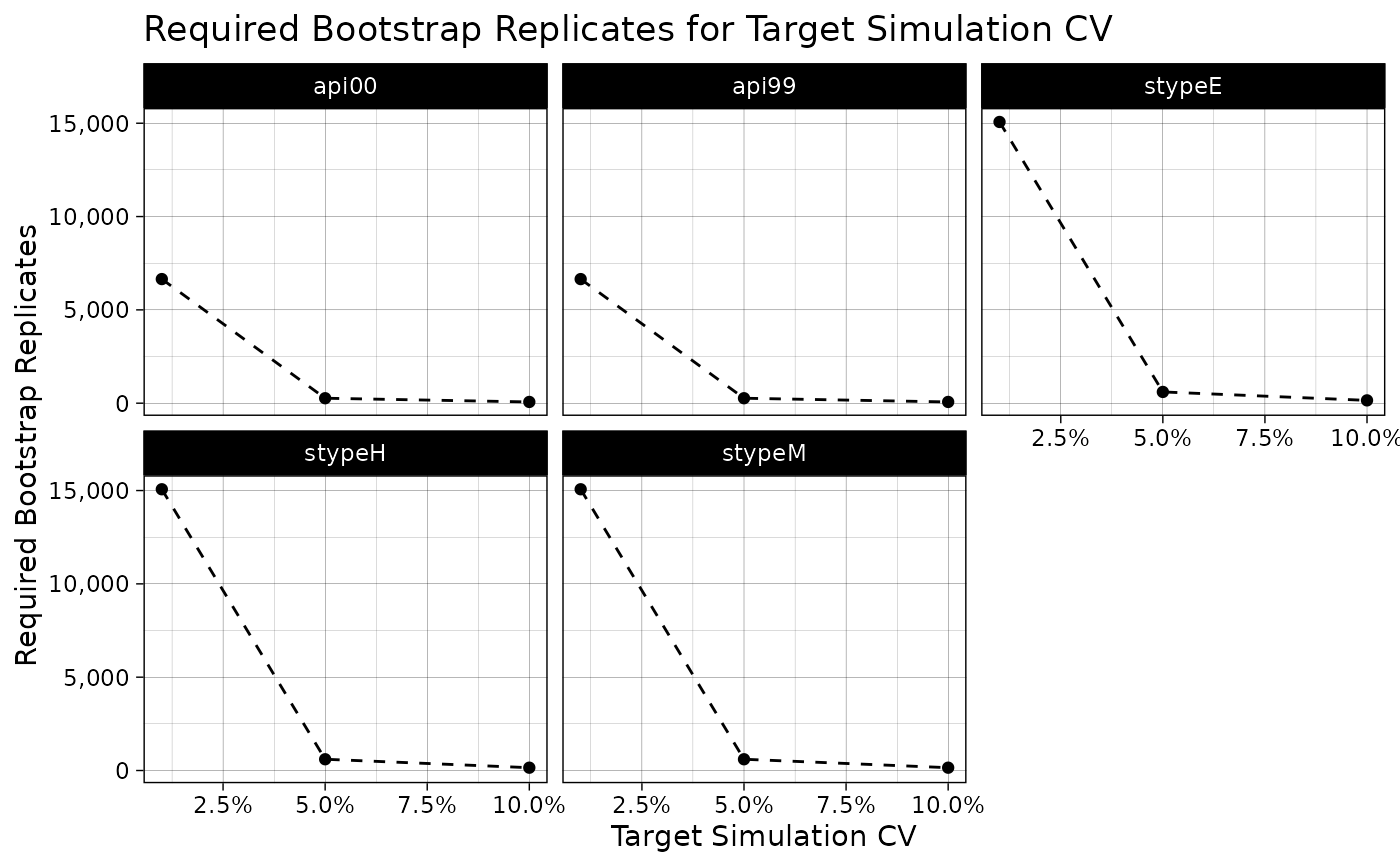
#> TARGET_CV MAX_REPS api00 api99 stypeE stypeH stypeM
#> 1 0.01 15068 6650 6649 15068 15068 15068
#> 2 0.05 603 266 266 603 603 603
#> 3 0.10 151 67 67 151 151 151
if (require('ggplot2')) {
plot(sim_cv_curve)
}
#> Loading required package: ggplot2
 ## For custom statistic
estimate_boot_reps_for_target_cv(
svrepstat = custom_statistic,
target_cv = c(0.01, 0.05, 0.10)
)
#> Warning: The elements of `svrepstat` are unnamed. Placeholder names (STATISTIC_1, etc.) will be used instead.
#> TARGET_CV MAX_REPS STATISTIC_1
#> 1 0.01 19781 19781
#> 2 0.05 792 792
#> 3 0.10 198 198
# }
## For custom statistic
estimate_boot_reps_for_target_cv(
svrepstat = custom_statistic,
target_cv = c(0.01, 0.05, 0.10)
)
#> Warning: The elements of `svrepstat` are unnamed. Placeholder names (STATISTIC_1, etc.) will be used instead.
#> TARGET_CV MAX_REPS STATISTIC_1
#> 1 0.01 19781 19781
#> 2 0.05 792 792
#> 3 0.10 198 198
# }